

What is Machine Learning?
Algorithm : a process or set of rules to be followed in calculations or other problem-solving operations, especially by a computer. - Google
Example : How much coffee should I drink before the test day to maximize my score?
>>> make a graph of how much coffee you drank -> test score
Coffee : 1 -> Score : 50
Coffee : 2 -> Score : 60
Coffee : 3 -> Score : 68
Coffee : 4 -> Score : 81
Prediction : drink 7 coffee -> Score of 100
oops! Your prediction of drinking 7 coffee -> Score of 100 was wrong. Why?
A : simply using mathematical equations for machine learning is widely wrong. Using deep learning would help. Deep learning is a part of machine learning
Problem Solving : when solving problems with machine learning, you can separate the solutions into two groups : regression and classification
Regression
In Regression, you need to define its inputs and outputs. For instance, the picture of a person (information) and the person's age in the image (output). When the result is continuous (like age, it increases from 1 to about 100), you use regression.
Classification
You use classification when your output is NOT continuous. For instance, how much time a student studies for the test (input) and whether the student failed (output). Here, the output is not continuous - it's either Fail or Success.
However, when there are more classes in the output, as the exact score of the test in the example above. Then, you use multi-class classification, or multi-label classification, where each class is each output. (A B C D F -> 5 classes)
Both
You can use both methods in some circumstances, like when you have to guess the RANGE of the person's age in the picture. Here, the output is both continuous and classifiable.
Three types of machine learning
Machine Learning can be categorized into three categories : supervised learning, unsupervised learning, and reinforcement learning.
Difference between supervised learning and unsupervised learning
Supervised learning has definite values as its output, while unsupervised learning has no definite outputs. In some way, supervised learning is somewhat more accurate.
Supervised Learning
Having inputs with annotations (ex. giving an apple picture with the annotation 'it's an apple.' computer will learn that the apple picture depicts an image of an apple.) It requires a lot of work as it needs tons of annotations.
Unsupervised Learning
Having inputs WITHOUT annotations (grouping algorithms : giving a picture of mixtures between apple and bananas -> computer categories apples to one group, and bananas to another group.) It takes a long time for the computer to learn this way. (Here are 100 different albums. Try to categorize them according to their similarities!)
Reinforcement Learning (Alphago)
Having rewards for actions the computer takes. It's a way for the computer (Agent) in its current state to learn how to get the highest reward by taking different actions.
Linear Regression
Example : Can we predict the test score by looking at how much coffee I drank the day before the test?
Formula of JUST the data given : H(x) = Wx + B
Cost Function (Loss Function) : the distance between the formula's graph and the data's graph (distance from the graph to the data^2 = error value)
Cost Function is used to determine whether the equation computer outputted is close to the data or not. It's a way for machines to reward themselves and decide it's following actions.
Prediction (Hypothesis equation) -> Cost Function -> determination
Multi-Variable Linear Regression
Same thing, but with more than one variables
Example : Can we predict the test score by looking at how much coffee I drank and how much time I studied the day before the test?
Variables : Study time and coffee
Gradient Descent Method
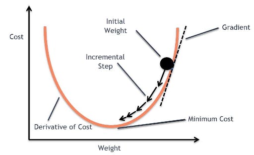
It's a way of moving a dot to the minimal point in order to optimize the cost (cost function). It will keep going as long as the method decreases the cost from the previous one.
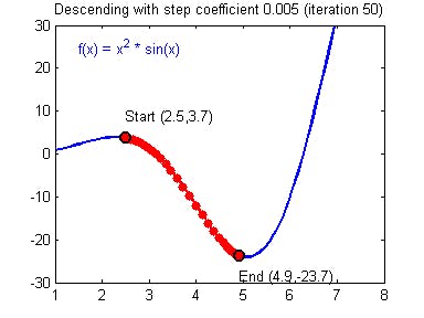
Iteration is how much the method was repeated.
Learning rate is the rate of how much the dot moves each time. The bigger the learning rate, the lesser time it takes. However, if the learning rate is too big, it may not be accurate and bounce up and back and not being able to find the minimal point for a long time (Overshooting). You need to set a decent learning rate in order to maximize productivity.
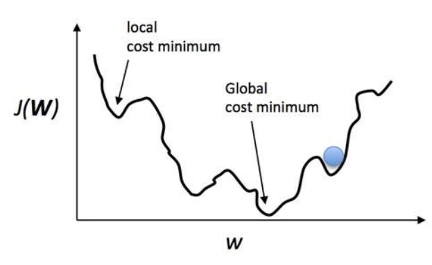
When you use the Gradient descent method, your dot may be stuck in the local minimal point, as when it moves a bit, the cost increases, and the computer thinks that it's the lowest point. It's the engineer's job to set a good hypothesis and the method to find the global minimum point.
Dataset Division
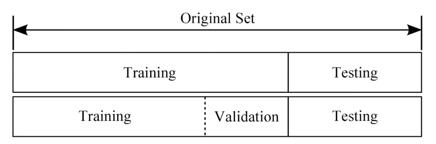
Training Set : It's where the computer is educated. It is approximately about 80% of the whole data set.
Validation Set : It's where your computer is validated. However, the model doesn't know what score they got in the validation set. It is approximately about 20% of the whole data set.
Test Set : This is where your computer gets tested in where it's used. This is totally different from the validation set since it doesn't matter whether it got a good score in the validation set or not; it's just about what it does in the actual environment.
Linear Regression Using Tensorflow
import tensorflow as tf

tf.compat.v1.disable_eager_execution()

x_data = [[1, 1], [2, 2], [3, 3]]
y_data = [[10], [20], [30]]

X = tf.compat.v1.placeholder(tf.float32, shape=[None, 2])
Y = tf.compat.v1.placeholder(tf.float32, shape=[None, 1])

W = tf.Variable(tf.random.normal(shape=(2, 1)), name='W')
b = tf.Variable(tf.random.normal(shape=(1,)), name='b')
Data for x,y -> placeholder (where data will be placed) -> define Weight and Bias (randomized)
hypothesis = tf.matmul(X, W) + b # Wx + b
cost = tf.reduce_mean(tf.square(hypothesis - Y))
optimizer = tf.compat.v1.train.GradientDescentOptimizer(learning_rate=0.01).minimize(cost)
Defining Hypothesis and cost function (gradient descent optimizer)
with tf.compat.v1.Session() as sess:
  sess.run(tf.compat.v1.global_variables_initializer())

  for step in range(50):
    c, W_, b_, _ = sess.run([cost, W, b, optimizer], feed_dict={X: x_data, Y: y_data})
    print('Step: %2d\t loss: %.2f\t' % (step, c))

  print(sess.run(hypothesis, feed_dict={X: [[4, 4]]}))
Repeating Gradient Descent method until the cost is minimized
Linear Regression Using Keras
import numpy as np
from tensorflow.keras.models import Sequential
from tensorflow.keras.layers import Dense
from tensorflow.keras.optimizers import Adam, SGD

x_data = np.array([[1], [2], [3]])
y_data = np.array([[10], [20], [30]])

model = Sequential([
  Dense(1)
])

model.compile(loss='mean_squared_error', optimizer=SGD(lr=0.1))

model.fit(x_data, y_data, epochs=100) # epochs (Plural)
Trials 100 times (epochs=100) minimizing cost function
Linear Regression Using Kaggle
Downloading Kaggle dataset in Google Colab
- Login to Kaggle
- Go to the Account Page (top right)
- Click on API - Create New API token and download kaggle.json
- Open kaggle.json in browser and copy username and key
- Paste username and key in the code below
import os
os.environ['KAGGLE_USERNAME'] = 'ericshindev' # username
os.environ['KAGGLE_KEY'] = '7e8c38399867d7c318135c93b4dbb1e9' # key
Downloading particular Dataset in Google colab
- Look for the dataset you want (ex. kaggle.com/ashydv/advertising-dataset)
- Click on [Copy API command] (Click on ... next to New Notebook)
- Paste it on the code cell below (Don't forget to put ! at the front)
!kaggle datasets download -d ashydv/advertising-dataset
Unzipping dataset
!unzip /content/advertising-dataset.zip
Single - Variable Linear Regression
from tensorflow.keras.models import Sequential
from tensorflow.keras.layers import Dense
from tensorflow.keras.optimizers import Adam, SGD
import numpy as np
import pandas as pd
import matplotlib.pyplot as plt
import seaborn as sns
from sklearn.model_selection import train_test_split
Loading Dataset
df = pd.read_csv('advertising.csv')
df.head(5)
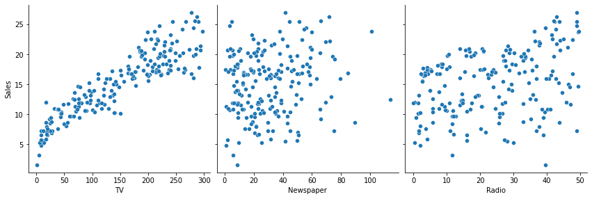
Glimpse of the Dataset
sns.pairplot(df, x_vars=['TV', 'Newspaper', 'Radio'], y_vars=['Sales'], height=4)
Result :
Reshape Dataset
x_data = np.array(df[['TV']], dtype=np.float32)
y_data = np.array(df['Sales'], dtype=np.float32)

print(x_data.shape)
print(y_data.shape)
x_data = x_data.reshape((-1, 1))
y_data = y_data.reshape((-1, 1))

print(x_data.shape)
print(y_data.shape)
Dataset Division
x_train, x_val, y_train, y_val = train_test_split(x_data, y_data, test_size=0.2, random_state=2021)

print(x_train.shape, x_val.shape)
print(y_train.shape, y_val.shape)
Train
model = Sequential([
  Dense(1)
])

model.compile(loss='mean_squared_error', optimizer=Adam(lr=0.1))

model.fit(
    x_train,
    y_train,
    validation_data=(x_val, y_val)
    epochs=100
)
Linear Regression
from tensorflow.keras.models import Sequential
from tensorflow.keras.layers import Dense
from tensorflow.keras.optimizers import Adam, SGD
import numpy as np
import pandas as pd
import matplotlib.pyplot as plt
import seaborn as sns
from sklearn.model_selection import train_test_split

df = pd.read_csv('advertising.csv')

x_data = np.array(df[['TV', 'Newspaper', 'Radio']], dtype=np.float32)
y_data = np.array(df['Sales'], dtype=np.float32)

x_data = x_data.reshape((-1, 3))
y_data = y_data.reshape((-1, 1))

print(x_data.shape)
print(y_data.shape)

x_train, x_val, y_train, y_val = train_test_split(x_data, y_data, test_size=0.2, random_state=2021)

print(x_train.shape, x_val.shape)
print(y_train.shape, y_val.shape)

model = Sequential([
  Dense(1)
])

model.compile(loss='mean_squared_error', optimizer=Adam(lr=0.1))

model.fit(
    x_train,
    y_train,
    validation_data=(x_val, y_val), # Validates after each epoch
    epochs=100 # epochs (plural)
)
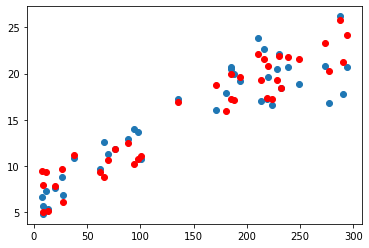
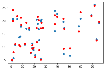
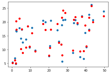
Graphs
Project colab.research.google.com/drive/1x_a6ajAD65..
My Result
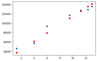
Thoughts
It was interesting to see how machines get to figure out the equation through processes, reducing its loss every time. I haven't gone through any local cost minimums, so I can't really say that I experienced every basic, but still, it was satisfying to see the graphs I've outputted using certain codes.