Logistic Regression

Why Logistic Regression?

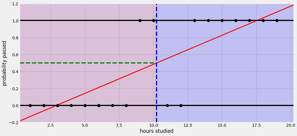
There are certain limits to linear regression. For example, the percentage of passing the test based on how long you studied the night before. In this problem, linear regression will go over / under the limits of percentage, like -10% or 110%, since it's a linear, endless function.

Linear Regression

Logistic Regression

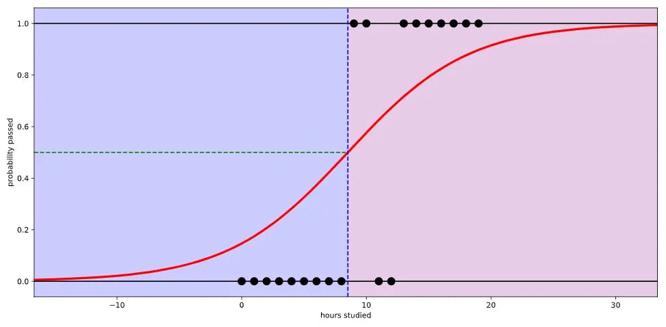
This s-curved function is called the sigmoid function, which is the prominent form of equation in logistic regression.

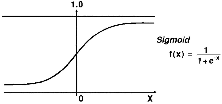
While linear regression's function looks like this: H(x) = Wx + b, the sigmoid functions looks like 1 / 1 + e^-(Wx + b). The cost function is more complex, however, my course didn't go through it as the lecturer focused more on the theories rather than maths.

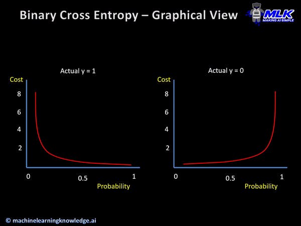
Cross entropy is a way of adjusting the graph to the actual points using the cost function. It is similar to the moving dots method (Gradient Descent Method) from linear regression. In Keras, you use binary_crossentropy in order to execute the method.

Multinomial Logistic Regression

Why Multinomial Logistic Regression?

Let's take the same example for the logistics regression, but except for this time you have to predict the grade, not the possibility of passing the test. Here, merely getting the percentage is not enough, in fact, it is unnecessary.

One-hot Encoding

One-hot Encoding is a way of indexing the classification in multinomial logistic regression. From the example above, let's divide the classes into five different ones: A, B, C, D, F. There are five classes, so we will have five booleans, in the form of 0s and 1s. Then, you plug the 1 (True) only in where you want to index them:

A: [1, 0, 0, 0, 0]

B: [0, 1, 0, 0, 0]

C: [0, 0, 1, 0, 0]

D: [0, 0, 0, 1, 0]

F: [0, 0, 0, 0, 1]

Softmax

Why Softmax?

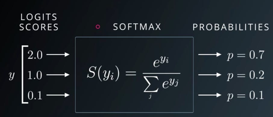
In Multinomial Logistic Regression, you cannot use the sigmoid function right away. You first need to get the logits from the linear regression, then the softmax converts the logit values into probabilities, adding up to 1. This adding up to one method is important since the one-hot encoding method also adds up to 1.

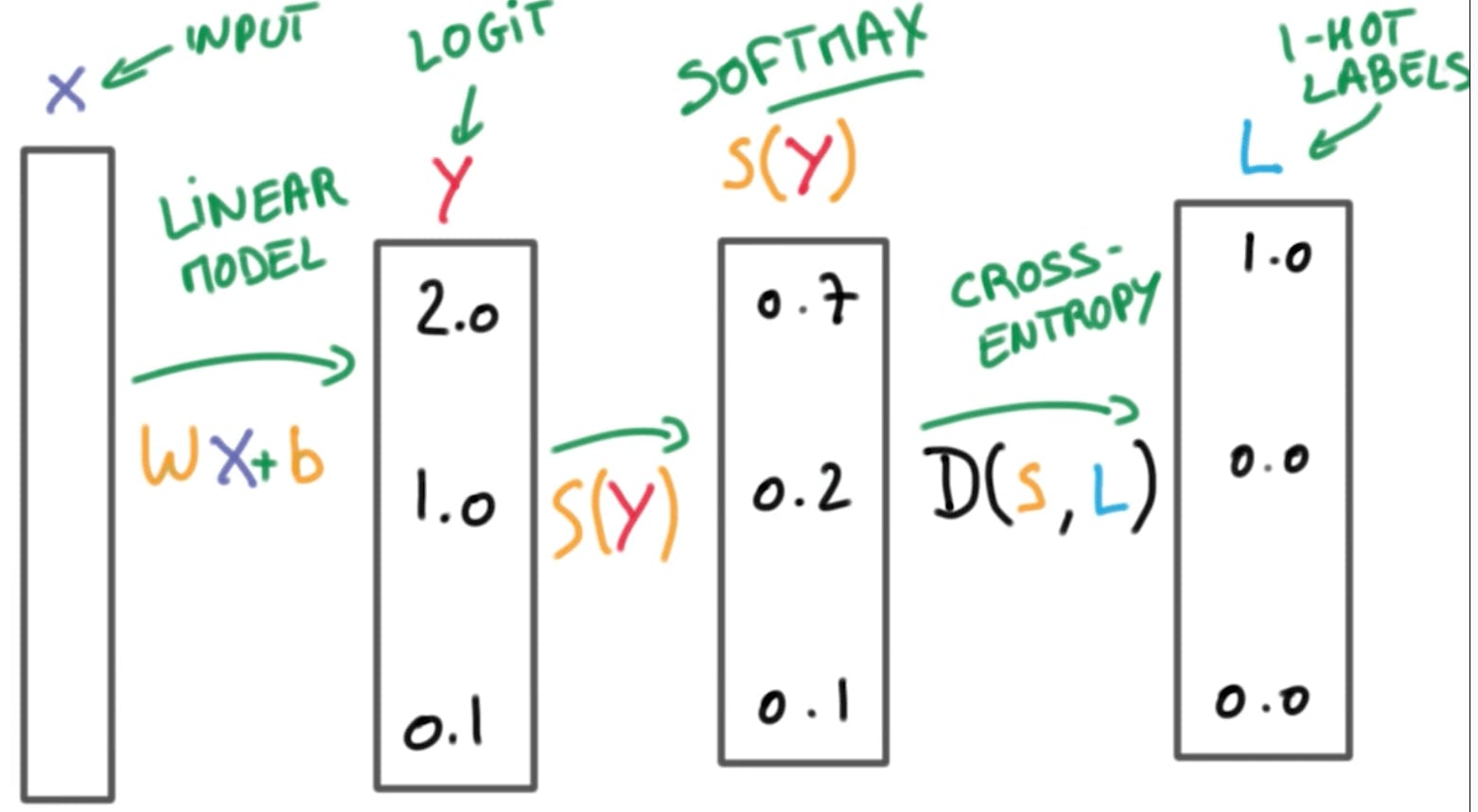
Imagine the graph below is the result of the softmax method: you still have to use the cross-entropy method to reduce the cost function, but here you execute another form of that: categorical crossentropy method. In Keras, you use categorical_cross-entropy to use this method.

Different Machine Learning models

Support Vector Machine (SVM)

When you have problems where you need to classify the objects, it is called the classification problem. The models used to solve such problems are called the Classifiers, which SVM is one of.

Let's imagine a machine has to classify between dogs and cats. You can use variables like the length of the animal's ears, and the animal's loyalty towards its owner. Now, in this graph, you will have many dots: what the machine needs to do is to draw a line, or a rectangle, that differentiates the dots that are cats from the dots that are dogs.

The bigger the margin, the better the accuracy. Now, it doesn't always have to be a 2D graph: you can always put more features in like the pitch of the animal's voice.

k-Nearest Neighbors (KNN)

Use the same example as the SVM. However, instead of drawing the support vector lines, KNN finds the nearest dot and identifies the dot according to the nearest one. For example, if animal A's plot is closest to animal B's plot, which is a cat, KNN identifies animal A as a cat.

Decision Tree

Literally, it is a tree of questions and decisions, like Does he have an ear longer than 3cm? Yes -> Is he loyal to his owner? No -> It is a cat.

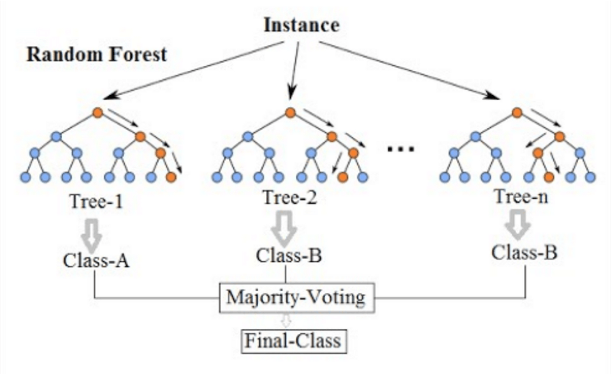
Random Forest

Random Forest is composed of several different decision trees, as one tree can be about ears and another one totally about its loyalty, and more. In the end, it identifies an object by the Majority of the decision tree's result. It is known for its accuracy, however, it is a pain in the butt for the programmers to sort out every decision trees.

Preprocessing

Preprocessing is so important that it usually takes up over 70 percent of the whole machine learning process.

Preprocessing is a way of filtering the data before the machine tests it. It deletes and saves what is important and what is negligible.

Let's say we are preprocessing the real-estate data with data like the area of the house, when it was built, how many floors, and how far away it is from the closet train station.

It is wrong to assume this: A's house is 30m^2 big, and B's house is 10km away from the train station, so B's house is more expensive. This is an example of taking different data types and comparing them.

It is also wrong to assume this: A's score is 50 out of 100, and B's score is 430 out of 500, so A's score is better. This is an example of falsely having the data's measures into comparison.

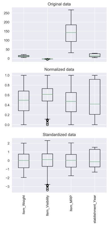
Normalization is classifying the categories to be within 0 and 1 to enable Logistic Regression, as logistic regression's graph has limits of 0 and 1

For example, 50 points out of 100 would be 0.5, and 50 out of 500 would be 0.1. This makes the second error above to be 'solvable.'

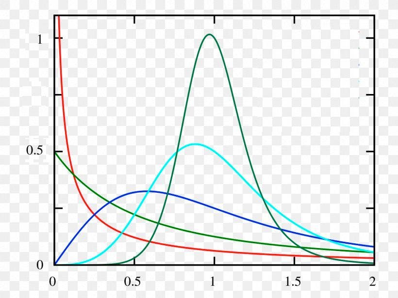
Standardization is making the graph standardized to a certain point so it's faster and easier for the machine to solve. Like the images below, standardization doesn't necessarily plot the data in the range of 0 and 1 but makes the graphs look similar to each other.

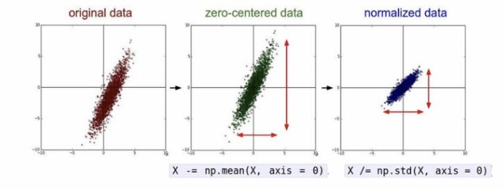
Preprocessing is important since it can greatly reduce the chance of falling into local minimums. It is best to use one of normalization or standardization, according to appropriate circumstances.

Logistic Regression in Google Colab

Downloading Dataset

import os
os.environ['KAGGLE_USERNAME'] = 'ericshindev' # username
os.environ['KAGGLE_KEY'] = '7e8c38399867d7c318135c93b4dbb1e9' # key

!kaggle datasets download -d heptapod/titanic

!unzip titanic.zip

Tensorflow and optimizers

from tensorflow.keras.models import Sequential
from tensorflow.keras.layers import Dense
from tensorflow.keras.optimizers import Adam, SGD
import numpy as np
import pandas as pd
import matplotlib.pyplot as plt 
import seaborn as sns
from sklearn.model_selection import train_test_split
from sklearn.preprocessing import StandardScaler

Loading Dataset (pandas)

df = pd.read_csv('train_and_test2.csv')

df.head(5)

Extracting data that we're going to use only

df = pd.read_csv('train_and_test2.csv', usecols=[
  'Age', 
  'Fare', 
  'Sex', 
  'sibsp', 
  'Parch', 
  'Pclass', 
  'Embarked', 
  '2urvived' 
])

df.head(5)

Previewing Dataset

sns.countplot(x='Sex', hue='2urvived', data=df)

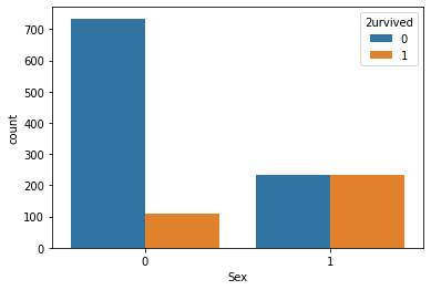
Over 700 males died and 100 males lived, and about 200 females survived and 200 females survived.

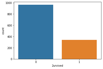
Checking the number of the survival class

sns.countplot(x=df['2urvived'])

Preprocessing - checking any null values

print(df.isnull().sum())

Age 0

Fare 0

Sex 0

sibsp 0

Parch 0

Pclass 0

Embarked 2

2urvived 0

dtype: int64

There are 2 null values in Embarked, so we're going to delete them.

print(len(df)) # number of data before deletion

df = df.dropna()

print(len(df)) # number of data after deletion

Alloting x and y values

x_data = df.drop(columns=['2urvived'], axis=1) # dropping the y value
x_data = x_data.astype(np.float32)

x_data.head(5)

y_data = df[['2urvived']]
y_data = y_data.astype(np.float32)

y_data.head(5)

Standardization

scaler = StandardScaler() # module you're using
x_data_scaled = scaler.fit_transform(x_data)

print(x_data.values[0])
print(x_data_scaled[0])

Dataset division (training sets and validation sets)

x_train, x_val, y_train, y_val = train_test_split(x_data, y_data, test_size=0.2, random_state=2021)

print(x_train.shape, x_val.shape)
print(y_train.shape, y_val.shape)

Testing

model = Sequential([
  Dense(1, activation='sigmoid')
])

model.compile(loss='binary_crossentropy', optimizer=Adam(lr=0.01), metrics=['acc'])

model.fit(
    x_train,
    y_train,
    validation_data=(x_val, y_val), 
    epochs=20 # trials 20 times
)

Multinomial Logistic Regression using Google colab

I will only plot out where it's different from the logistic regression. Downloading data from Kaggle is still the same.

Tensorflow and Modules

from tensorflow.keras.models import Sequential
from tensorflow.keras.layers import Dense
from tensorflow.keras.optimizers import Adam, SGD
import numpy as np
import pandas as pd
import matplotlib.pyplot as plt
import seaborn as sns
from sklearn.model_selection import train_test_split
from sklearn.preprocessing import StandardScaler
from sklearn.preprocessing import OneHotEncoder # yes, it is the one-hot encoder defined above.

One-hot Encoding (This is after the standardization)

encoder = OneHotEncoder()
y_data_encoded = encoder.fit_transform(y_data).toarray()

print(y_data.values[0])
print(y_data_encoded[0])

Testing

model = Sequential([
  Dense(3, activation='softmax') # use softmax, and the number is 3 not 1
])

model.compile(loss='categorical_crossentropy', optimizer=Adam(lr=0.02), metrics=['acc']) # its categorical_crossentropy, not binary!

model.fit(
    x_train,
    y_train,
    validation_data=(x_val, y_val),
    epochs=20 
)

Thoughts

It's getting harder and harder, and the codes are getting more complex, but it's fun to see how I'm getting able to process these codes and solve more complex problems. From having simple linear graphs, I extended my limits to having sigmoid functions in the calculation. I'm very proud of myself, and thanks to my online instructor, I think I'm starting to think about seriously studying this field, with proper maths and all that.